Post-AGI Australia: Fiscal Transition Modelling © 2026 by Kent Fitch is licensed under CC BY 4.0![]()
![]()
Draft 12.0 - 30 April 2026, Kent Fitch, kent.fitch@projectcomputing.com
Accompanying interactive model: Draft 12.0 artefact
Accompanying model technical detail and history: Draft 12.0 summary
Post-AGI Australia: Fiscal Transition Modelling © 2026 by Kent Fitch is licensed under CC BY 4.0![]()
![]()
Only a crisis — actual or perceived — produces real change. When that crisis occurs, the actions that are taken depend on the ideas that are lying around. That, I believe, is our basic function: to develop alternatives to existing policies, to keep them alive and available until the politically impossible becomes the politically inevitable.
Milton Friedman, 1972
Milton Friedman was a monster, but he wasn't wrong about this.
If the huge investment in AI turns out to be justified and delivers massive productivity gains, causing
then a wage-ratio variable GST
could result in a better economic outcome for almost all Australians and a measurably more equal society.
This report documents the motivations, modelling strategies, and evolving findings of a fiscal transition model designed to explore Australia's potential path into an economy transformed by Artificial General Intelligence (AGI): a post-AGI economy. The model is a scenario tool rather than a forecast: it examines how a broad, unified fiscal system could absorb rapid technological productivity gains, large-scale labour displacement, and deflationary price dynamics while maintaining social stability.
The model's core policy structure combines:
The model includes an industry-level supply-side model (18 sectors), household micro-outcomes (24 ABS-and-ATO-derived household types: 20 ABS-grounded plus 4 high-income types calibrated to ATO 2022-23 individual percentile data), and a decomposition of non-tax revenue sources into 14 categories sourced from the PBO Australia's Tax Mix dataset's 16-category state/territory/local breakdown. The model can run in either Retail Sales Tax (RST) mode on final consumption or, by default, in Goods and Services Tax (GST) mode with input credits, using ABS Input-Output (IO) tables aggregated to the model's 18 sectors to compute gross GST, input credits, and net GST.
The main findings to date:
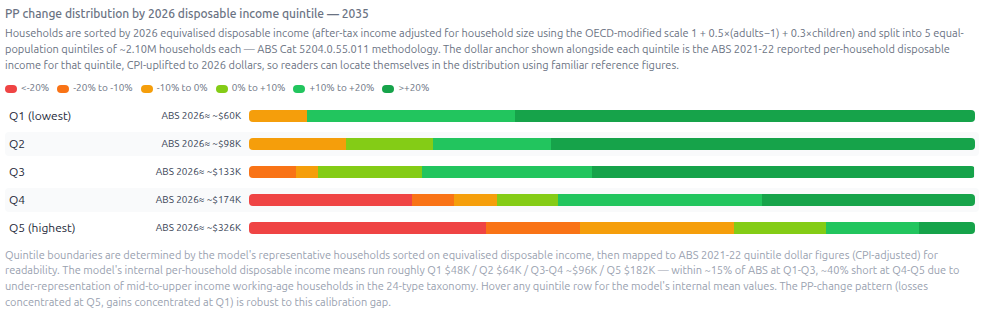
The disposable-income quintile chart (ABS Cat 5204.0.55.011 methodology) shows the Gini reduction's mechanism clearly: losses concentrate at the top quintile (Q5 households, ABS 2026≈$326K disposable, have 33% of population in the >20% PP-loss tail) while gains concentrate at the bottom (Q1 households, ABS 2026≈$60K disposable, have 90% in positive PP bands).
The net effect is to move Australia from its current inequality levels to a profile more similar to Scandinavian countries.
Aside from the obvious uncertainty about AGI capability and timing, the model's strongest uncertainties lie in the calibration of industry AGI exposure, the behavioural responses of labour supply and consumption under AGI-induced price deflation, the integrity of the company tax base under AGI-enabled transfer pricing, and the size of the consumer-side incidence of variable GST on foreign-owned firms.
Future work could prioritise:
Vast resources continue to be invested into AI research and commercialisation. Anthropic CEO Dario Amodei believes AGI will be achieved by 2028. DeepMind CEO Demis Hassabis is more conservative, giving it until 2030. Both are at the forefront of AI research and commercialisation, and although both have skin in the game, rapid advances in the field are occurring across a wide front and AGI could emerge from any number of research teams.
AGI is not a certainty, any timeline is necessarily speculation, and the effect of AI on company structures and employment is debated, for example, The AI Layoff Trap (Falk & Tsoukalas), What Will Be Scarce? (Alex Imas), Employment data shows the early signs of AI job disruption are already here (Clinton Free) and Why the A.I. Job Apocalypse (Probably) Won’t Happen (Ezra Klein). However dismissing Amodei and Hassabis and at least the possibility of widespread economic disruption seems as reckless as ignoring the warnings of climate scientists in the 1990s. Whether the timeframe is 2 or 10 years, the potential prospect is the same. As characterised by Amodei: "Cancer is cured, the economy grows at 10% a year, the budget is balanced - and 20% of people don't have jobs."
As AI-powered and then AGI-powered cycles both increase its capability and decrease its cost, economic reasons and opportunities for employing human labour of almost all kinds could well shrink along with the rapidly increasing GDP. Without rethinking fundamental assumptions of our society, wealth will become increasingly concentrated, and with it, power and inequity. AGI will likely lead to an "age of abundance" from rapid advances in materials, medical treatment, manufacturing, agriculture, and unforeseeable improvements in education and entertainment. But it could also result in disastrously uneven access to productivity gains, widespread economic and social disruption, and consequent social pressures.
Without an equitable plan for the transition to a post-AGI economy, both gross social disruption and delays to a generally better future are possible. For something as significant and reasonably likely to happen so quickly as AGI, there is relatively little discussion or policy preparation. Surely it is better to canvas, evaluate and rehearse responses before they are needed.
The question is not when AGI will arrive, that remains uncertain, but whether Australia's fiscal architecture could survive the shock if it did, and what replacement architecture might work. Milton Friedman's observation that crises are managed using the ideas already "lying around" provides the motivation: if AGI does arrive on the timeline suggested by leading AI researchers, then analysed and credible policy options must exist before the disruption arrives, not after.
The central motivation for this model is to explore a plausible fiscal structure for Australia under conditions of rapid AGI adoption. The assumed conditions are:
The model is intended to answer the following policy questions:
Consider an accountancy practice whose business is primarily preparing tax returns. They may currently take 2 hours and charge $600 for a typical individual return: 1.5 hours talking to the customer, eliciting relevant details, and communicating the result; 30 minutes entering and checking data and lodging it with the ATO. The accountant's charge-out rate of $300/hour covers their wage, superannuation, leave provisions, insurance, accreditation, premises, cleaning, IT, and so on.
It seems reasonable to assume that the accountant could use AGI to automate the entire process, from customer communication to checking and lodgement, with the accountant merely supervising and quality-checking. The accountant's time may fall from 2 hours to 15 minutes, or just $75 of accountant "time" (and less if the necessity for leave and super provisions is reduced). The cost of the AGI may be just $5. Competitive pressures could reduce the cost of preparing this tax return from $600 to $80: effectively, AGI has deflated the price. It is likely that far fewer accountants will be required: if this practice previously needed 8 people, they now need just 1. It is hard to imagine demand for accounting services will be so elastic that all 7 displaced accountants will find equivalent employment. The cost reduction from $600 to $80 is clearly a boon for the consumer, but an uneven benefit: there are now out-of-work accountants, unable to add their incomes to the economy. So how can this benefit be spread so that AGI's productivity is welcomed rather than (ultimately futilely) resisted?
The model treats the fiscal system as whole-of-government (Commonwealth + States + Local), focusing on aggregate sustainability rather than intergovernmental distributions. It tracks 18 industries, 24 household types (20 ABS-grounded plus 4 high-income, with a further 4 renter-sensitive variants), and produces year-by-year fiscal balances, debt trajectories, and purchasing-power distributions across the 2030–2035 transition period. All figures are in constant 2026 Australian dollars. The model's 2026 tax baseline incorporates the 2025-26 income year stage 3 brackets, low income tax offset and the Medicare levy with low-income threshold.
The model is a deterministic, scenario-based simulation with three interacting layers:
Earlier drafts of the model layered Keynesian-style multiplier rounds (~$400–450B at 2035 at default settings) and a separate fund-spending GST line on top of the macro GST. Both were removed in Draft 11 as double-counting. The reasoning is straightforward: in equilibrium, household consumption equals household-share-of-consumption (defaults to 60%) x total-GDP, regardless of which sources fund it (wages, GDI, fund returns, dissaving). The macro GST taxes that consumption exactly once. Real fiscal statements never isolate "multiplier revenue" or "induced GST" because, once equilibrium is reached, all induced flows are baked into observed GDP, wages, profits, and tax collections.
This represents a significant philosophical shift. The earlier multiplier-style framing produced more flattering headline numbers but obscured what was actually being asked of the policy package. The current framework makes the trade-offs transparent: if GDI levels and tax rates cannot balance without phantom multiplier revenue, the model should reveal that, not hide it.
The model still distinguishes the parts that do require explicit accounting. For example, the investment-response capex feedback (§6.1), which adds genuinely new GDP composition rather than re-counting existing spending, from the parts that don't. See §6.5 for the equilibrium-consumption discussion in full.
The model is implemented as an interactive artefact (available here) with adjustable policy levers and detailed outputs. The visible UI exposes 35 sliders (income floor, tax/consumption parameters, productivity & macro, tax arbitrage, asymmetric feedbacks, behavioural elasticities, and personal income tax brackets) and approximately 215 hardcoded calibration constants documented in the constants reference file.
The artefact's main panels are:
This report is intended for readers with a working knowledge of Australian fiscal policy and public economics. It is intended to provoke discussion. It is total folly to imagine the model is "accurate". Even something seemingly as simple as the Commonwealth's removal of FBT on EVs, initially modelled as costing the budget $70 million in 2025-26, proved difficult for a Treasury full of modelling boffins - their latest cost estimate for 2025-26 is $1.35 billion. Instead, the goal is to test plausible directions and measure the shape of their outcomes and their robustness to inevitable uncertainty and the model maker's naivety and ignorance (including "unknown unknowns").
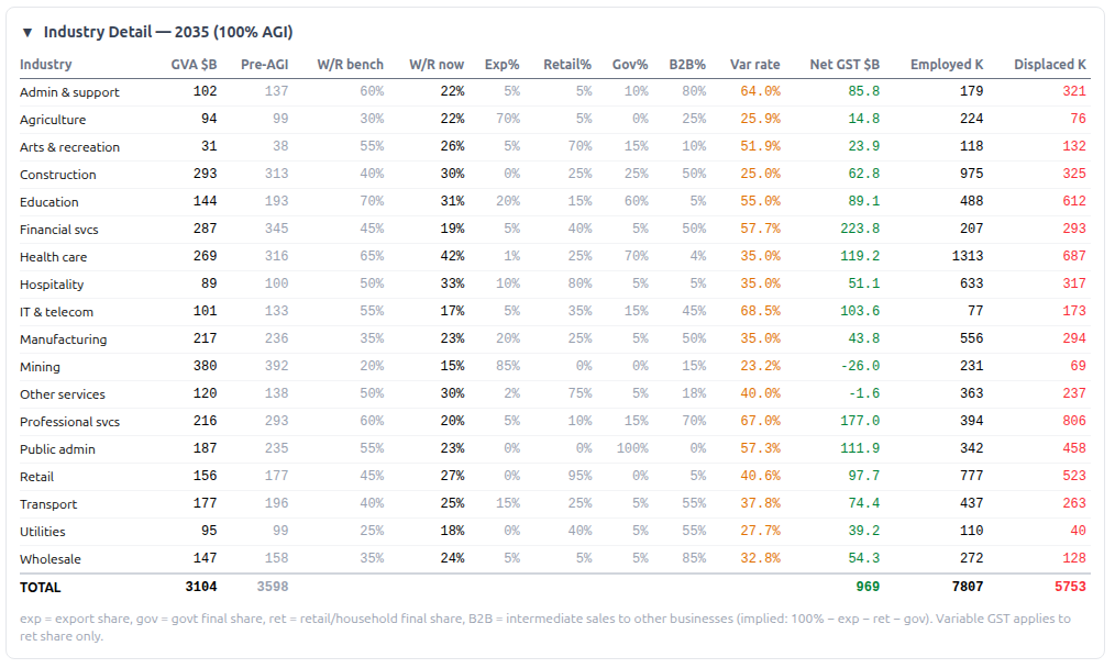
The central economic challenge of AGI is the speed and breadth of labour displacement. Unlike previous waves of automation, which affected narrow occupational categories over decades, AGI has the potential to substitute for labour, including cognitive labour, across most industries simultaneously. The model estimates that at full adoption in 2035, approximately 42% of current employment (about 5.7 million jobs) would be displaced in total across the 18 modelled industries, with exposure rates ranging from 70% in IT and telecommunications to 25% in construction.
This is not a prediction. It is a scenario designed to stress-test fiscal policy under extreme but plausible conditions. If AGI displaces even half this amount, existing income support systems designed for frictional and cyclical unemployment at 4–6% would be overwhelmed. JobSeeker payments, which currently support roughly 800,000 recipients at a cost of approximately $15 billion per year, could not scale to millions of displaced workers without either fiscal collapse or severe benefit reduction. Falling demand for goods and services would spiral throughout the economy.
Australia's tax system is heavily dependent on labour income. Personal income tax and payroll tax together constitute approximately 55% of total government revenue. As AGI substitutes for human labour, this base erodes. The displaced workers earn less (or nothing), reducing income tax collections. Businesses that replace workers with AI systems pay no payroll tax on those systems. Meanwhile, the businesses themselves may be more profitable (if they can still find paying customers and aren't subject to market competition), but profits are mobile, and Australia's company tax base is already subject to significant transfer-pricing erosion. That is, increasing company tax is unlikely to be an effective mechanism: in competitive markets, AGI will add little to company profits (with the AGI gains going to consumers), and in uncompetitive markets, companies will organise to earn profits in offshore tax regimes.
AGI-driven automation reduces production costs which, left to market, will manifest as a balance between higher profits and lower prices. Businesses operating in oligopolistic or regulated markets could capture all the value while those in highly competitive markets may capture none. But the trend will be towards falling prices and price deflation that increases the real purchasing power of any fixed-dollar transfer. A Guaranteed Daily Income of $105/day in 2035, while modest in nominal terms (~$38k/year), purchases significantly more in a deflated market.
This deflationary dynamic is central to the model's fiscal logic: the government can afford to pay lower nominal transfers because each dollar buys more, while simultaneously collecting larger nominal revenues from the variable GST on AI-augmented output.
Beyond fiscal solvency, the model asks whether households at every point in the income distribution can maintain or improve their purchasing power relative to 2026. This is measured through a Purchasing Power (PP) index computed for each of 24 household types (plus 4 renter variants), with displaced workers modelled separately from those who retain employment. A PP index of 100 means a household has equivalent purchasing power to 2026; below 100 means the household is worse off.
The model's Personal Scenario Calculator allows any household to enter their own financial details and see a direct 2026 vs 2035 comparison under the model's current settings.
Many younger people feel that the economic playing field is tilted against them. It isn't just that housing requires an unprecedented share of income; many incur much higher HECS debts than their parents and grandparents. True, each generation inherits vast infrastructure: roads, hospitals, universities, legal institutions, power networks largely paid for by their forebears. But increasing privatisation and uneven maintenance mean the current generation inherits a smaller bounty than previous generations took for granted. Many see the tax system as perpetuating intergenerational disadvantage, citing negative gearing, capital gains discounts, and superannuation tax concessions as disproportionately benefiting older people.
This model revamps the tax system and abolishes superannuation and disincentives to employment such as payroll tax and leave entitlements. It does so because the ends they serve are met by the means of the lifetime Guaranteed Daily Income. GDI is received from birth, at a lower rate until age 18. Younger people will obviously receive more GDI over the course of their lives than older people.
The model's default settings reduce the model's income Gini from 0.222= in 2026 to 0.18 in 2035, an 18% reduction. The reduction is driven by the GDI floor and the abolition of regressive structural features (super tax concessions, payroll tax, the 50% CGT discount). It is a structural property of the policy package, not a fine-tuning result.
The model's Gini is still conservative compared to ABS Gini estimates because the 24 household-type taxonomy compresses within-type income dispersion (e.g. the model's Q5 mean of $182K disposable vs ABS's $326K). The directional finding of substantial reduction in Gini survives across calibrations; the absolute level remains a lower bound on the official inequality measure.
The redistribution of foreign-firm GST incidence into household PP (§6.4) makes the regressive incidence of foreign-firm passthrough show up correctly in the Gini metric. Even with that effect included, the Gini reduction holds.
The disposable-income quintile chart shows households sorted by 2026 equivalised disposable income, split into 5 equal-population quintiles, displayed against ABS-reported per-household disposable income anchors (~$60K / $98K / $133K / $174K / $326K in 2026 dollars). It shows the redistributive pattern that drives Gini compression.
The model replaces all existing income support programs (JobSeeker, Age Pension, Parenting Payment, Family Tax Benefit, and most other transfers at approximately $153 billion per year) with a universal Guaranteed Daily Income. Every adult receives at least the daily GDI, 365 days of the year, with the transfer reduced dollar-for-dollar when daily salary earnings exceed the GDI rate. Children receive a flat daily amount regardless of household income.
The GDI differs from a Universal Basic Income in one critical respect: it is a top-up, not a flat payment. An adult earning a salary of $500/day receives zero GDI. An adult earning $50/day on a day they work also receives $55 of GDI on that day (if the rate is $105/day), plus the full daily rate on non-work days. This design preserves work incentives at low income levels while providing a realistic floor.
The default model ramps the adult GDI from $80/day in 2030 to $105/day by 2035. The child rate ramps from $20/day to $45/day. At $105/day the annual GDI is $38,325, which sits below the default tax-free threshold of $45,000, meaning GDI-only recipients pay zero income tax. The increasing adult GDI through the transition reflects growing fiscal capacity as AGI revenue ramps up and deflation increases purchasing power.
The GDI is taxable and integrated into standard income tax brackets.
Rationale. A guaranteed income is essential under large-scale displacement. The model treats GDI not as charity but as the primary economic stabiliser, and, in the equilibrium framework, as a redistribution mechanism rather than a fiscal stimulus. AGI raises productivity; the GDI plus the wage-ratio variable GST redirect a share of those gains from automated profits and overseas AI providers to displaced workers.
The key revenue mechanism. Each business's variable GST rate is determined by its wage-to-revenue ratio relative to a pre-AGI sector benchmark:
Variable rate = Maximum levy × (1 − actual wage ratio ÷ pre-AGI benchmark wage ratio)
The maximum levy is a model parameter; the model default is 100%, a setting deliberately chosen to sit comfortably inside the no-deployment-distortion range described in §5.3.
A business that maintains pre-AGI employment levels pays 0% variable GST. A fully automated business pays the maximum levy. There is no self-assessment: the rate is mechanically derived from the ratio of reported wage expenses to reported revenue, both of which are already disclosed to the ATO through existing BAS and payroll reporting.
This design has three advantages over alternative automation taxes:
At full AGI adoption with a 100% maximum levy, variable GST collections reach several hundred billion dollars per year and become the largest single revenue item. It is the mechanism that replaces the eroded income tax base.
The variable GST is applied to each industry's deflated output value × final-consumption share × demand multiplier, and is computed in either RST mode (B2B and exports zero-rated; consumer pays the full rate at point of final sale) or, by default in GST mode, using ABS IO tables to compute gross GST, input credits, and net GST.
Scope clarification: The variable GST applies to industries including financial services (40% retail share) and IT & telecom (35% retail share), which are largely GST-exempt or input-taxed under current Australian law. The model's variable GST therefore functions as a broad-based VAT on consumer-final services and goods, not a "Retail Sales Tax" in the narrow sense. The terminology in earlier drafts ("RST") obscured this. This is a deliberate design feature: the post-AGI economic transition requires a tax base shift from labour to consumption, which means broadening the consumption tax to include currently-exempt services where labour income is otherwise vanishing. Globally, NZ taxes financial services partially; Singapore and several EU states tax most services. Treasury has periodically modelled financial-services GST inclusion at $20–40B per year in revenue at current rates. The implementation requirement is real, extending Australian GST coverage to currently-exempt categories is a significant policy change.
The variable GST mechanism interacts with firm-level economics in a way that earlier drafts ignored. At very high levy values, an AGI-using firm's consumer price would exceed a pure-human-labour competitor's price, and a profit-maximising firm wouldn't adopt AGI in the first place. Draft 11.3 introduced a per-firm break-even formula:
r_break = 0.65 × L × (1 + b) / (1 − 0.65 × L × maxAGI-levy)
where L is industry labour intensity and b is the AGI-import cost share. A new "Adoption price sensitivity" slider (default 60%, range 0–100%) controls how strictly the cap "binds", accommodating within-industry firm heterogeneity.
The implication is significant. Past about 150% maxAGI-Levy, the cap binds in most industries and additional levy produces no further revenue but suppresses an increasing share of AGI deployment. The maxAGI-levy setting is therefore a deployment/disruption knob that affects revenue. In the policy framing, "how aggressively do we want AGI deployed?" is the meaningful question; "how much revenue can we raise through the levy?" is largely answered by the underlying labour-intensity × levy rate distribution and is bounded above regardless of nominal rate.
The model default of 100% maxAGI-levy sits comfortably inside the no-distortion range. Variable GST revenue is still substantial (~$652B at peak in GST mode, net of input credits) but no AGI deployment is fiscally suppressed.
The model broadens the consumption tax base to include all goods and services, removing current exemptions for fresh food, health, education, residential rent, and financial services. This increases the effective coverage from approximately 50% of consumption to 85% (the residual 15% covers items difficult to tax, such as imputed rent on owner-occupied housing).
The base GST rate is set by slider (default 12%, range 10–25%). Variable GST stacks on top of base GST in industries with AGI exposure.
For renter households, a deliberate asymmetry applies: base GST is added to rent (with pass-through assumed: landlords with pricing power pass the GST on to tenants, the more economically realistic assumption than landlord absorption), but the variable GST component is not applied to rent because landlords have no AGI-displacement wage benchmark.
The model assumes the superannuation pool ($6T) is transferred in 2030 to a single government-managed investment fund. Returns are distributed and taxed as ordinary personal income, stacking on GDI and wages. There is no concessional tax treatment of any kind.
Fund assumptions:
These assumptions produce ~$70B-$90B per year in personal income tax on distributed returns.
Former account holders retain nominal ownership of their assets. All returns are distributed annually and taxed as ordinary income. Realised capital gains are immediately distributed as capital gains income to the holder, reduced by a CPI discount (the ratio of the prevailing CPI at purchase and sale). All holders, regardless of age, are free to withdraw their capital partially or completely, or to add capital. There is no concessional tax treatment of any kind. The modelled drawdown of $700B of the fund over the transition years acts as a significant buffer, making savings available to households in transition.
The rationale is fivefold:
Progressive brackets are kept but with a high tax-free threshold. The model removes the Medicare levy and treats GDI as taxable income. The current default brackets are:
|
Income bracket |
Marginal rate |
|
$0 – $45K |
0% |
|
$45K – $90K |
30% |
|
$90K – $120K |
35% |
|
$120K – $150K |
40% |
|
$150K + |
45% |
These are flatter at the top than the 2025-26 stage 3 brackets and rely on the GDI to provide the bottom-end progressivity that the income tax system used to deliver. An interesting finding (§7.3 below) is that top-bracket extension is fiscally near-zero: the income distribution simply doesn't have enough mass at the top end for personal income tax progressivity to matter at the macro level.
Rationale. The tax base should focus on total income rather than wages alone. Progressive income tax claws back much of the GDI transferred to high-income earners. Capital gains are taxed as income, with CPI-indexed cost base adjustment (the pre-1999 method) replacing the current 50% discount.
Employers are not responsible for any leave provisions (holiday, sick, personal), redundancy provisions, or superannuation contributions. Along with the abolition of payroll tax, these changes remove disincentives to employing people whilst the GDI provides an income safety-net. The labour cost of an employee becomes their pre-tax wage and nothing else.
Employers need to compete with the GDI to attract employees.
Five feedback mechanisms and two methodological refinements have been added in recent drafts, each addressing a real-world phenomenon.
During major productivity events, for example the ICT boom 1995–2002, where capex ran ~1.5pp of GDP above trend, firms invest heavily in deployment infrastructure. AGI deployment is plausibly such an event: integration with existing systems, robotic systems, data-centre buildout, and capacity expansion in sectors that complement AGI all generate direct activity.
The model adds an investmentBoost parameter (default 2.0% of GDP at full AGI adoption, range 0–5%). At each transition year, additional capex of investmentBoost × realGDP × af flows into the economy and produces:
Cumulative contribution over the six-year transition: approximately +$48B. 2035 endpoint improvement: approximately +$18B per year. No material effect on Gini (the new workers are middle-income).
Two channels with opposite fiscal directions:
Channel A: Variable GST collection on imports (positive). The earlier importLeakage parameter treated imported consumption as pure leakage: both base and variable GST lost. This is overly conservative: Australia's 2017 low-value-import GST reform already collects base GST from cooperating offshore providers via EDP/agent registration. A post-AGI Australia could extend variable GST collection to imports of the same industry categories by analogous mechanisms.
Two parameters control the channel:
At the model defaults, Channel A contributes ~$140B per year at 2035, ramping with adoption.
Trade-policy second-order effect. A high variable GST levy on imported AGI services is effectively a soft trade barrier on AGI-intensive imports. WTO-defensible because it's a non-discriminatory consumption tax (applied to domestic and imported equally), but it could provoke retaliatory measures from major trading partners (US tech companies are the largest exporters of AGI services to Australia). This is not a model-internal problem but a real-world implementation risk that's part of the policy package.
Channel B: Profit shifting via transfer pricing (negative). An earlier draft treated the company tax base as fully collectable, which is known to be optimistic. ATO transfer-pricing audits suggest $15–25B per year in current losses (~5–10% of the $140B 2022-23 company tax base). AGI makes IP and "services" more easily mispriced because:
The mechanism scales the baseline profit-shifting rate (default 7%, range 0–20%) by (1 + 0.5 × af), reaching 10.5% at full AGI adoption. At the model defaults, Channel B costs approximately $30B per year by 2035.
Combined effect. Net contribution at model defaults: approximately +$110B per year at 2035. Cumulative net contribution over the transition: approximately +$278B.
When GDI provides an unconditional floor, some workers will exit voluntarily. UBI trial evidence (Finland, Stockton, Kenya) suggests 2–5% of secondary earners and lower-wage workers withdraw participation. The model adds a voluntaryWithdrawal parameter (default 3%, range 0–8%).
Mechanism: exited workers lose their wage income tax, gain full GDI (rather than GDI top-up), and reduce consumption (which also reduces GST). At default 3% × full adoption, approximately 0.24M workers exit by 2035, costing approximately $15B per year fiscally. Sensitivity is bounded: even at 8% (the UBI evidence ceiling), the cost rises only to about $24B per year.
The offsetting wage-rise dynamic (labour scarcity raising wages for those who remain → more income tax → less GDI top-up) and the deflation-reduces-required-income effect are NOT modelled. Net direction is well-established (negative); magnitude is upper-bounded by the simple model. Implementing the offsetting feedbacks would push the model's fiscal cost closer to −$8 to −$10B per year but doesn't change the qualitative finding.
Variable GST levied on foreign-owned firms operating in Australia is partly passed through to Australian consumers via prices, rather than being absorbed by foreign capital. Two parameters control the mechanism:
At the model defaults, this produces approximately $78B per year in consumer-borne foreign-firm GST at peak. Fiscally neutral: the GST is collected either way, just from a different ultimate payer. Distributionally regressive: consumer-borne incidence falls more heavily on lower-income households who consume a larger share of disposable income.
The current model redistributes the burden across the household types via spend rate (newSR), making it correctly regressive. Bottom-quintile households absorb proportionally more of the foreign-firm GST passed through to consumers.
Future calibration improvements (further upper-tail expansion, per-quintile basket weighting) would amplify the regressive effect without changing the directional finding.
The previous "fiscal multiplier" was conceptually motivated by the idea that GDI is "new spending introduced by the policy". But GDI is not new spending in the comparative-statics sense: it is a redistribution from displaced wage income to transfer income, plus a top-up financed by company tax / variable GST / overseas AI provider levies / deficit. Households still consume; the funding source has shifted. The model now treats this correctly via a single equilibrium-consumption GST calculation.
Fiscal impact of removing the multiplier: the 2035 fiscal balance worsened by approximately $400–450B and peak debt rose. If GDI levels and tax rates cannot balance without phantom multiplier revenue, the model should reveal that, not hide it. The Draft 11 default settings (consShare raised from 50% to 60% to reflect the actual ~56% national accounts figure plus a modest upward shift expected as GDI shifts income toward higher-MPC households) compensate partially.
The same equilibrium argument applies to the previous separate fund-spending GST line (fund-funded household spending is part of total household consumption already taxed in the macro GST). Removed in Draft 11; fiscal impact ~$15–20B per year revenue reduction.
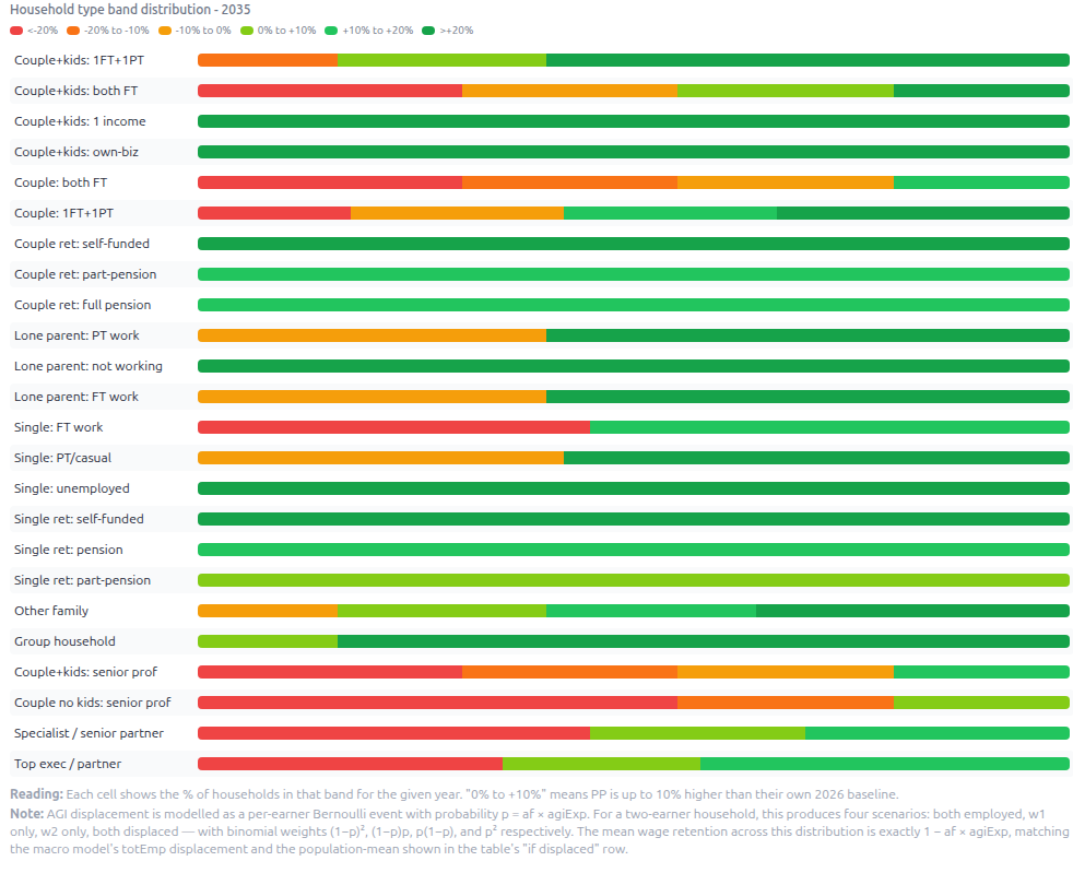
Earlier drafts modelled within-type purchasing-power dispersion as a smooth multiplicative spread (scale factors 0.7–1.3 with weights 10/20/40/20/10%) centred on the population-mean displaced wage scale 1 − af × AGI exposure. The intent was to show that not all households of a given type experience the same outcome. The actual effect was to make the band chart inconsistent with the household outcomes table: the dispersion never reached scale 1.0 (full employment), so working types' band distributions never showed any households in the positive PP bands, even when the table's "employed" row for those types showed strongly positive PP. For "Couple: both FT" at 2035 default settings, the table showed employed PP=114 and "if displaced" PP=83, but the band chart placed 100% of these households below PP=100.
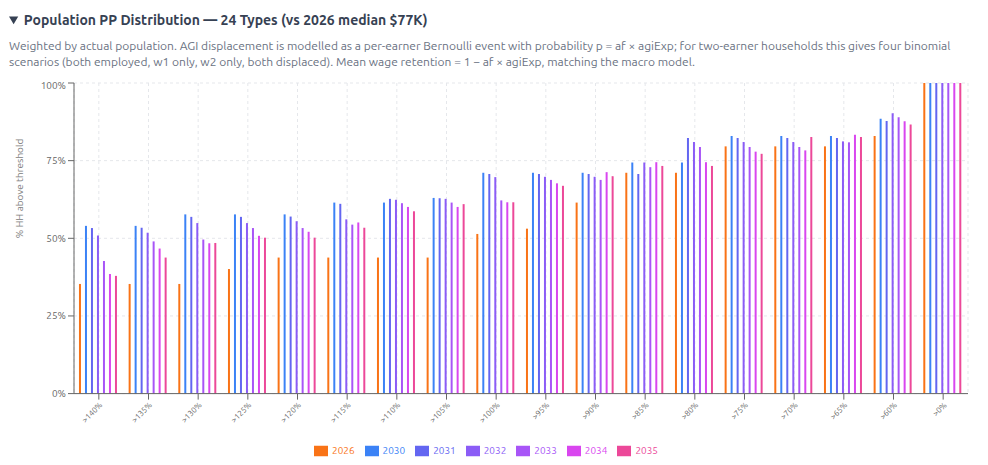
Draft 11.8 replaced the multiplicative dispersion with a per-earner Bernoulli model. For each working household, each earner is independently displaced with probability p = af × AGI exposure. For two-earner households, this produces 4 binomial scenarios:
The mean wage retention across the binomial is exactly 1 − p, which matches the macro model's totEmp displacement and the household table's "if displaced" row by construction. The table's "if displaced" row therefore correctly represents the population-mean displaced outcome (the binomial expectation), while the band chart now exposes the spread around that mean.
The model also corrects a related minor inconsistency: wageScale (GDP growth flowing partly to wages, ≈1.095 at 2035 default) is now applied in the band-chart calculation, matching its application in the household table's calcOneHH. Without this, the both-employed binomial scenario for "Couple: both FT" computes as PP ≈106 (band 0/+10%) rather than the table's PP=114 (band +10/+20%), a difference that affects which band the scenario lands in.
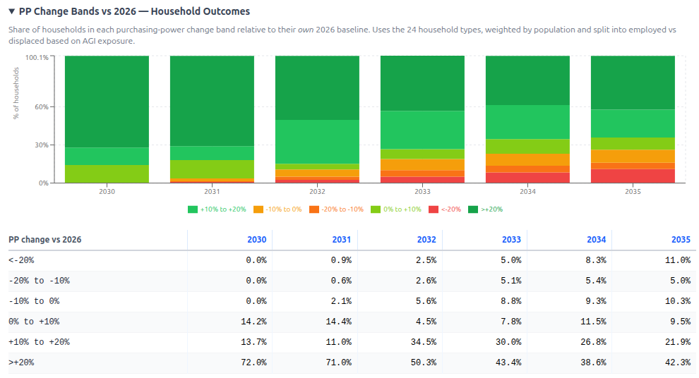
The fix changes the band-chart, PP-Change-Bands, and Population-PP-Distribution views, and also propagates into the Gini metric.
The model now better represents AGI-driven displacement. The 30% of "Couple: both FT" households in the <-20% band corresponds to the both-displaced binomial weight (p² for p=0.55), a structural property of the displacement probability, independent of tax rates or other policy parameters. Tax-rate changes in higher brackets shift PP values within scenarios but cannot push the binomial weights themselves; to influence the bottom of the distribution, policy levers must affect the GDI floor or the displacement probability itself.
The taxonomy gap. The 20 ABS-derived household types used through Draft 11.8 peaked at "Couple+kids: both FT" with a 2026 gross household income of $207K. ABS Cat 5204.0.55.011 (2021-22) reports the top quintile's mean gross disposable income at $288K (~$326K in 2026 dollars after CPI adjustment). The model was therefore under-representing the genuine upper tail of the Australian household distribution. This was acceptable when the model's primary outputs were macro fiscal trajectories (which are driven by WAGE_GROUPS and totEmp, not HH_TYPES), but became problematic once the binomial within-type displacement (§6.6) and ABS-comparable distributional reporting (§4.6) made the household-level distributional analysis a first-class output.
The fix. Draft 11.9 added 4 new household types in a new category code HI ("HIGH INCOME"), calibrated to ATO Taxation Statistics 2022-23 individual percentile thresholds:
|
Type |
hhK |
gross 2026$ |
AGI exposure |
Calibration |
|
Couple+kids: senior prof |
200 |
~$295K |
0.55 |
Both adults at ATO 95th individual percentile |
|
Couple no kids: senior prof |
100 |
~$290K |
0.55 |
Same income profile, no children |
|
Specialist / senior partner |
150 |
~$405K |
0.45 |
Primary earner at ATO 98th percentile; specialist judgment work less automatable |
|
Top exec / partner |
50 |
~$605K |
0.35 |
Primary earner at ATO 99th percentile; executive role hardest to automate, but equity comp still AGI-exposed |
Total: 500K HH (5% of total). Total non-RV HH_TYPES rises from 9.98M → 10.48M, within the ABS estimate of ~10.5M private households for 2026.
Macro fiscal numbers are unchanged: 2035 endpoint (+$25B), cumulative balance (−$1,399B), debt (88% of GDP), and employment (7.81M). calcModel reads WAGE_GROUPS (8-group ATO-calibrated individual wage distribution) and totEmp (industry-derived from labour-cost share × AGI displacement). HH_TYPES is not used in calcModel; only the household-level views (table, band charts, Gini) consume it.
The income-band chart. v11.8's chart bucketed households into 7 nominal-dollar gross income bands (<$30K, $30-60K, ..., >$200K). This couldn't be reconciled with ABS reporting because ABS quintiles are defined by equivalised disposable income (sorted) but displayed as per-household disposable income: apples-to-oranges with our nominal-gross bands.
Draft 11.9 replaced this with proper ABS Cat 5204.0.55.011 methodology. Households are sorted by 2026 equivalised disposable income: after-tax income divided by the OECD-modified equivalence factor 1 + 0.5×(adults−1) + 0.3×children. This adjusts for household size to enable fair comparison: a single retiree on $40K and a couple-with-2-kids on $90K have similar equivalised income (around $40K each) because the family's income supports more people. Households are then split into 5 equal-population quintiles of ~2.1M each.
The chart displays the ABS 2021-22 per-household disposable income, CPI-uplifted to 2026 as the dollar anchor for each quintile: ~$60K / $98K / $133K / $174K / $326K. Readers locate themselves in the distribution using familiar reference figures rather than the model's internal computed values (which are smaller: Q5 mean $182K vs ABS $326K, and would invite confused dismissal).
The model's internal per-household disposable income means are roughly $48K (Q1), $64K (Q2), $96K (Q3), $96K (Q4), $182K (Q5). This is within ~15% of the ABS-equivalent at Q1-Q3 but ~40% short at Q4-Q5. The gap reflects under-representation of mid-to-upper income working-age households (the taxonomy has no representative type between Couple+kids 1FT+1PT at $122K disposable and Couple+kids both FT at $166K disposable). The PP-change pattern (losses concentrated at Q5, gains concentrated at Q1) is robust to this calibration gap.
The Gini effect. Adding upper-tail mass increases inequality measures in both 2026 and 2035, but more so in 2026 (since AGI displacement compresses upper-tail PP harder than lower-tail).
Draft 12.0's recalibration of HH_TYPES child counts to ABS Census 2021 averages also slightly changed modelled Gini.
At the default settings, the 6-year transition trajectory is:
|
Year |
AGI adoption |
GDP |
Budget Balance |
Cumulative |
Total Employment |
|
2030 |
0% |
$3,200B |
−$445B |
−$445B |
13.45M |
|
2031 |
10% |
$3,302B |
−$417B |
−$862B |
12.81M |
|
2032 |
30% |
$3,421B |
−$315B |
−$1,178B |
11.54M |
|
2033 |
55% |
$3,562B |
−$179B |
−$1,357B |
9.98M |
|
2034 |
80% |
$3,725B |
−$69B |
−$1,426B |
8.58M |
|
2035 |
100% |
$3,912B |
+$25B |
−$1,399B |
7.81M |
Existing 2030 gross debt $2,050B + cumulative transition deficit $1,399B = 2036 cumulative gross debt of $3,449B (88% of GDP). The 2035 endpoint surplus of $25B/year is modest but achieves transition financing balance: post-2035, the system runs structural surpluses that pay down the transition debt over approximately 10–15 years.
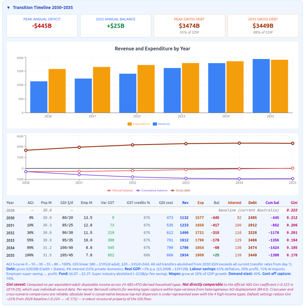
The "transition deficit" framing matters. Critics will say "you're running $1.4T cumulative deficit over 6 years" - yes, but every dollar of that deficit funds an asset (workforce transition, debt-financed infrastructure, AGI deployment) that pays returns from 2035 onwards. The 2035 endpoint structural surplus offers a path that post-transition, the system is fiscally viable.
The trajectory is contingent on:
The binomial within-type displacement model reveals that the right way to read distributional outcomes is within household types as well as between them. For each working two-earner household type, the binomial produces four scenarios: both employed (weight (1−p)²), one earner displaced (weight 2p(1−p) split between the two single-earner cases), and both displaced (weight p²) with the mean wage retention exactly matching the macro model.
For "Couple: both FT" (childless, AGI exposure 0.55) at 2035 default settings, the type with the worst aggregate outcome, the binomial decomposes roughly as:
|
Scenario |
Weight |
Wage retention |
Approx PP |
|
Both employed |
20% |
100% |
~112 (→ +10/+20% band) |
|
w1 only (w2 displaced) |
25% |
56% |
~88 (→ −20/−10% band) |
|
w2 only (w1 displaced) |
25% |
44% |
~80 (→ −20/−10% band) |
|
Both displaced |
30% |
0% |
~56 (→ <−20% band) |
The population-mean PP for this type is approximately 81, close to the household table's "if displaced" row at PP 82 (which, by construction, is the population-mean displaced outcome). But the modal experience for these households is one of the four binomial scenarios, not the mean. Roughly 20% of these households retain full employment and gain meaningfully; 30% are fully displaced and face severe loss.
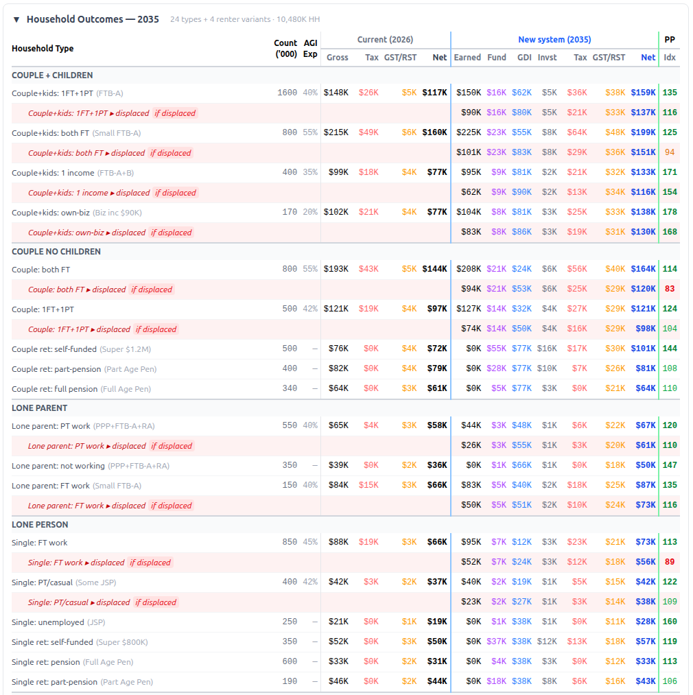
Across the 24 household types:
The renter variant households are not explicitly shown in the Household Band PP Distribution graph, but on average, the general Household Outcomes table shows their PP outcomes as positive.
The Gini reduction holds across all reasonable parameter settings. It is a structural property of the GDI floor combined with the abolition of regressive features (super tax concessions, payroll tax, the 50% CGT discount).
The population PP distribution chart makes the redistribution mechanism visible using ABS-comparable equivalised disposable-income quintiles. Households are sorted by 2026 equivalised disposable income (per the OECD-modified equivalence factor 1 + 0.5×(adults−1) + 0.3×children, which adjusts for household size) and split into 5 equal-population quintiles of approximately 2.10M households each, following ABS Cat 5204.0.55.011 methodology. Each quintile is anchored to ABS 2021-22 reported per-household disposable income for that quintile, CPI-uplifted to 2026 dollars, so readers can locate themselves using familiar reference figures.
|
Quintile |
2026 disposable income (ABS anchored) |
<-20% |
-20% / -10% |
-10% |
0% |
+10% |
>+20% |
|
Q1 (lowest) |
~$60K |
0% |
0% |
8.0% |
0% |
28.6% |
63.4% |
|
Q2 |
~$98K |
0% |
0% |
13.4% |
12.0% |
16.2% |
58.4% |
|
Q3 |
~$133K |
0% |
6.5% |
3.0% |
14.3% |
23.5% |
52.6% |
|
Q4 |
~$174K |
22.5% |
5.7% |
5.9% |
8.5% |
28.1% |
29.3% |
|
Q5 (highest) |
~$326K |
32.6% |
13.0% |
21.2% |
12.7% |
12.8% |
7.7% |
The pattern is unambiguous: gains concentrate at the lower quintiles and losses at the upper. Q1 has 63% of households in the best PP-gain tail (>+20%) and zero households in any negative band; Q2 and Q3 follow with 58% and 53% respectively in the >+20% tail. Q4 splits roughly two-thirds positive, one-third negative, with 22.5% in the worst loss tail. Q5 inverts: 33% in the worst tail, 67% in negative bands overall, only 8% in the >+20% gain tail. This is the redistributive pattern that drives the Gini reduction. The losers are predominantly childless dual-earner FT couples and FT single workers with high AGI exposure; the gainers are predominantly retirees, lone parents, PT workers, and lower-paid single-earner households, all benefiting from the GDI floor.
With the 4 ATO-calibrated high-income types added in Draft 11.9, the chart now covers the full population rather than truncating at the bottom ~95%. A residual calibration gap remains: the model's internal per-household disposable income means run roughly Q1 $48K, Q2 $64K, Q3-Q4 ~$96K, Q5 $182K, which is within ~15% of ABS reference incomes at Q1-Q3 but ~40% short at Q4-Q5 due to remaining under-representation of mid-to-upper income working-age households in the 24-type taxonomy. The qualitative redistributive pattern (losses concentrated at Q5, gains at Q1) is robust to this calibration gap.
Implication for policy design. The bottom-of-distribution tail (fully displaced households of high-AGI-exposure types) is where targeted transition support is most needed. A household-composition-specific GDI top-up for childless dual-earner displaced households, a temporary wage-replacement scheme for fully displaced single FT workers in high-exposure industries, or means-tested transition payments triggered by employment loss would address the binomial tail without disturbing the broader policy architecture.
A surprising finding from a model sensitivity sweep: extending the top tax bracket from 45%@$150K to 55%@$250K shifts the 2035 fiscal balance by less than $1B per year. Even more aggressive top-bracket changes (e.g. 50%@$200K) contribute only ~$5B.
The reason is the income distribution. After the model's recalibration to ATO 2018-19 percentile data, only 1% of taxpayers are above $350K and only 5% above $200K. Group 6 (6% of workers, ~$175K) and Group 7 (4%, ~$250K) are too thin a slice to matter at the macro level. The household types that hit those brackets ("Couple: both FT" at ~$180K combined, "Couple ret: self-funded" at ~$60K si × 2 adults) are split across two adults so individual brackets bind weakly.
Implication. Top-bracket extension is a political signal, not a fiscal lever. If revenue is the goal, the real levers are:
Top-bracket extension and other tax progressivity tweaks contribute under $5B individually.
The per-firm break-even cap analysis (§5.3) reframes the maxAG-levy slider. Past about 150% maxAGI-levy, the cap binds in most industries; additional levy produces no additional revenue but suppresses an increasing share of AGI deployment. At the model default of 100% maxAGI-levy, no AGI deployment is fiscally suppressed, so the variable GST is operating in its "deployment-neutral" range.
The reframed policy question: how aggressively do we want AGI deployed? The 100% setting is a deliberate choice not to discourage deployment; pushing to 110% or 120% would still be inside the no-distortion range but would start to produce small adoption-suppression effects in the highest-AGI-exposure industries (IT, financial services, professional services).
Removing GST-free categories (food, education, health, rent, financial services) materially changes outcomes:
The implementation requirement is real: extending Australian GST to currently-exempt categories (financial services, healthcare, education, residential rent) is a significant policy change. NZ taxes financial services partially; Singapore and several EU states tax most services. The variable GST scope clarification (§5.2) means this isn't optional: it's part of the mechanism.
The model sets the cost of AI service at 15% of gross labour savings, and assumes all these services are imported. At full adoption, approximately $70 billion per year flows offshore to pay for AI services. This is a permanent structural change in Australia's current account: the country was already a net importer of technology services, but AGI dramatically increases the scale.
The AI import cost interacts with variable GST via Channel A of the tax arbitrage mechanism (§6.2). Foreign AI providers serving Australian businesses have zero Australian wages, meaning they attract the maximum variable GST rate on any Australian-facing output. The import enforcement mechanism is what makes this credible: at default 80% collection × 75% basket factor, approximately 60% of variable GST that would otherwise be lost on imports is recovered, contributing about $140B per year at 2035.
The 15% of labour savings paid to overseas providers is also 15% that doesn't circulate in the Australian economy and hence doesn't generate further GST, company tax, or domestic consumption. The fiscal multiplier weakens as a result, compounding the effect of declining domestic employment.
The industry AGI exposure rates (maxAGI factors ranging from 0.25 for construction to 0.85 for IT and telecommunications) are among the model's most speculative inputs. They determine both the displacement trajectory and the variable GST revenue for each industry. Financial services at 80% maxAGI on a ~$256B GVA base generates the largest single industry contribution to variable GST. Healthcare (35%) could be much higher if diagnostic AI proves transformative, or much lower if regulatory and trust barriers slow adoption. Construction (25%) could rise significantly with autonomous machinery.
The model assumes 65% of labour cost savings from AGI adoption pass through to consumers as lower prices. This is reasonable for competitive industries but likely too generous for oligopolistic ones. Australian markets in banking, telecommunications, supermarkets, and energy are highly concentrated. If passthrough is only 40%, deflation is smaller, the real value of GDI is lower, and variable GST collections change (the tax base is larger but the purchasing power benefit is smaller).
The S-curve assumption (0% → 100% over 6 years) is aggressive. If adoption takes 10–15 years rather than 6, the transitional deficit period extends, peak debt is higher, and the interest cost compounds over a longer period. Conversely, slower adoption gives more time for labour market adjustment, potentially reducing GDI costs below what the model projects.
The 3% default for real GDP growth from non-AGI sources, plus a 2pp AGI productivity bonus at full adoption (slider range 0–5pp), are assumptions, not forecasts. If AGI produces primarily cost savings rather than new output categories, real GDP growth could be much lower (0 – 1.5% baseline + lower bonus), with severe implications for every revenue line that scales with GDP. Conversely, it could be reasonably anticipated that AGI will lead to new discoveries, inventions and optimisations across fields as diverse as agriculture, material science, education, health care and robotics leading to very significant improvements in productivity and GDP. The model's sensitivity to this combined parameter is high: each 1pp of AGI productivity bonus contributes approximately $90B to 6-year cumulative balance and $45B to 2035 endpoint.
Default settings: 25% import leakage of base consumption, but 80% collection of variable GST on imports of AGI-intensive categories via the §6.2 Channel A mechanism. The proposed enforcement mechanism (payment-layer withholding at Australian banks and card processors, extending the 2017 low-value-import GST regime) is untested at AGI scale. Lower collection or higher leakage would tighten the fiscal position significantly.
The model assumes company tax collections are maintained at 30% of a growing profit base, with a 7% baseline profit-shift rate growing to 10.5% at full AGI adoption (§6.2 Channel B). In practice, AGI makes transfer pricing trivially easy. If the effective profit-shift rate is materially higher than the modelled growth path, for example, 12% or 15% baseline, then the company tax base could erode further. Possible counter-measures (turnover-based alternative minimum tax, Pillar Two enforcement) are not modelled.
The model default of 70% government efficiency capture combined with a weighted average of 23.4% AGI amenability across services contributes approximately $162B per year at peak which is a meaningful contributor to the headline result. ±30% calibration uncertainty translates to roughly ±$50B per year fiscal swing. The headline framing could be: "Subject to government capturing 70% of a 23% weighted AGI amenability across services, contributing ~$160B/year to fiscal balance at peak."
The current amenability values reflect an assumption that AGI primarily automates administrative and information-processing work, with limited reach into hands-on services (Healthcare patient care, Defence operations, Aged care direct support). Plausible counter-arguments: AI-enabled diagnostics, robotic surgery, and AI tutoring could push Healthcare and Education amenability higher; embedded AI in defence systems could push Defence higher.
The maxAGI factors (0.25–0.85) are the model's most speculative inputs. They are not derived from a formal methodology but from informed judgement about the proportion of each industry's labour that could plausibly be substituted by AGI. The factors drive both displacement (and hence GDI cost) and variable GST revenue. A 10-percentage-point change in maxAGI for a large industry like financial services ($256B GVA) shifts variable GST by tens of billions of dollars.
Section 6.3 models voluntary withdrawal as a single-direction effect (workers exit, fiscal cost rises). The offsetting wage-rise dynamic (labour scarcity raises wages for remaining workers → more income tax → less GDI top-up) and the deflation-reduces-required-income effect are not modelled. Net direction is reliable; magnitude is upper-bounded.
Section 6.4 redistributes a default 12% of variable GST (= 30% foreign firm share × 40% consumer incidence) into household PP via spend rate. The 40% consumer-incidence assumption is a single calibration parameter. At 60% incidence, consumer-borne GST rises to ~$117B per year and the regressive Gini effect is more pronounced; at 20%, the effect halves. The model does not yet apply per-quintile basket weighting to this redistribution, which would amplify the regressive direction.
Beer sales have always attracted significant excise and since 2000, GST as well. Everyone is free to brew their own beer: the ingredients are cheap and the process is easy. Similarly, it seems very likely that anyone will be able to acquire their own computing hardware and AI software, and run an AGI at home, its outputs unseen and untaxed by the variable GST, with comparatively trivial costs for hardware and power.
But just as home brewing and bread-making are simple and economic, most people willingly pay the extra cost of commercial products. Running your own AGI to displace commercial services will have less friction and fewer disruptions to leisure time than beer or bread-making, and it is unclear how large the benefits will be compared to the costs and advantages of relying on "branded" services.
The model currently has no equivalent to the current very low tax-free threshold for unearned income by children ($416). As such, it would motivate adults to shift investments to their children. Similarly, the large tax-free threshold (default $45K) and its level above the maximum GDI ($38K) would motivate tax avoidance and minimisation by moving investments from higher earners to relatives receiving only the GDI. Both effects chip away at the ability of the system to fairly tax and redistribute.
Moving super from a highly tax-concessional environment of industry and retail funds to a low-cost but tax-neutral government fund will have many highly motivated critics. Not least the super "industry" that skims $30B in costs and fees from the public. Not least the high earners who have been encouraged by successive government policies to use super more as tax minimisation than a retirement savings vehicle. Not least retirees or near-retirees whose expectations of zero-taxed pension income will now attract marginal income tax rates, although they will also be paid the full GDI (considerably more than the pension they probably didn't even qualify for) and purchasing-power modelling shows most will be better off.
Perhaps most vocal will be the SMSF members who have moved what would normally be private businesses such as the family farm into an SMSF for clear tax minimisation, only to find that "management" of their super assets has moved from the SMSF to the government fund (although the owners remain as they always were: the beneficiaries of the SMSF). They will be free to "buy back" their farm and remove it from the fund, but any CPI-adjusted capital gain will be attributable as taxable income. Transition arrangements may be required for a small number of special cases.
But for most people, the GDI and equity "deal" that the abolishment of super is part of may be portrayed as successfully as "the Accord" was, which from 1983 to 1992 established the superannuation system. Persisting with tax distortions exemplified by the current super system increases the difficulty of achieving an efficient and equitable economy.
Under the binomial within-type displacement model, a better way to think about transition support is by within-type binomial scenario, not by aggregate household-type means. The two types with the most concerning aggregate outcomes are "Couple: both FT" (childless dual professionals, mean PP ~81) and "Single: FT work" (mean PP ~89). Both face high concentrated AGI exposure (AGI exposure 0.55 and 0.45 respectively) without the buffering provided by child GDI or a non-working second adult.
The deeper concern is the binomial tail across all high-exposure working types: roughly 30% of dual-earner FT households (childless or with kids) face the both-displaced scenario, with PP loss substantially worse than 20%; ~45% of single FT workers face the displaced-only scenario with similar severity. The mean PP for these types is closer to break-even than the worst-case scenario suggests, because the both-employed scenario (~20% of dual-earner households) lifts the average.
Targeted transition support is therefore better-aimed at the binomial tail than at the type mean. Possible mechanisms include:
These instruments would address the binomial tail without disturbing the broader policy architecture, and would be naturally self-targeting (only triggered by actual displacement events rather than membership of a particular household type).
GST collection underpins the fiscal viability of the large GDI transfers in the model. The payment-layer enforcement mechanisms must reliably collect GST from onshore businesses and from businesses that move offshore whilst serving Australian customers. The default 80% import-levy collection rate (§6.2 Channel A) reflects high but achievable compliance; significantly lower rates would tighten the fiscal position.
The model ignores several phenomena:
These omissions do not invalidate the model but should be kept in mind when interpreting results.
Several policy insights emerge:
The model provides a coherent, transparent framework for thinking about fiscal sustainability in a post-AGI Australia. It shows that solvency is possible at moderate, defensible settings, and that distributional outcomes can be substantially improved, but distributional outcomes can also diverge significantly across household types.
The model's value is not in prediction but in structured exploration. It helps clarify which levers matter most (GDI rate, maxAGI-levy in the moderate range, base GST, government efficiency capture, productivity bonus), which are largely cosmetic (top-bracket personal income tax extension), where trade-offs arise (variable GST as deployment dial vs revenue lever), and what data gaps must be closed before serious policy decisions can be made (industry AGI exposure calibration; foreign-firm consumer incidence empirics; voluntary labour withdrawal under deflation).
These findings are preliminary and intentionally transparent. The model is open-source. All assumptions are documented, all parameters are configurable (although some only in the model's code, not the exploration user interface), and the interactive tool allows users to explore alternative scenarios. The objective is not to propose a definitive policy framework but to provide a structured basis for thinking about fiscal architecture in a world where the relationship between human labour and economic output may be fundamentally altered.
Australia can afford this transition, but only by aggressively taxing AGI deployment, broadening the GST base to currently-exempt categories, and accepting a transition-financing deficit during 2030–2035 that pays down over the following decade.
This model and its settings are an initial exploration of the challenge and opportunity of a post-AGI economy. It is offered as a contribution to a vessel of "ideas lying around" that we should be actively filling, ready to be ransacked for the time when the impossible becomes inevitable.
|
Parameter |
Value |
Sensitivity |
|
Adult GDI ramp |
$80 → $105/day |
High — drives expenditure |
|
Child GDI ramp |
$20 → $45/day |
Low — small cost share |
|
Max AGI levy |
100% |
Moderate-high in 0–120% range; saturates above ~150% (§5.3) |
|
Base GST |
12% |
Medium — ~$10B per 1pp |
|
Company tax |
30% |
Medium |
|
Import leakage |
25% |
High; partly offset by §6.2 Channel A |
|
Real GDP growth |
3% p.a. |
Very high — scales all revenue |
|
AGI productivity bonus |
2pp at full adoption |
Very high — ~$45B per pp at 2035 endpoint |
|
Investment response |
2.0% of GDP |
Medium — ~$10B per pp at 2035 |
|
Govt efficiency capture |
70% |
Medium — ~$5B per 5pp |
|
Other rev AGI sensitivity |
50% |
Low–Medium |
|
AGI adoption |
S-curve, 6 years |
Very high — determines timing |
|
Starting gross debt |
$2,050B |
High — drives interest costs |
|
Interest rate |
4% |
Medium–High |
|
Competitive passthrough |
65% (hardcoded) |
High — drives deflation and var GST base |
|
Additional profit share |
20% (hardcoded) |
Medium — drives company tax |
|
AI service import share |
15% (hardcoded) |
Medium — economic leakage |
|
Adoption price sensitivity |
60% |
Medium |
|
Levy demand elasticity |
50% |
Medium |
|
Demand price elasticity |
40% |
Medium |
|
Import levy collection |
80% |
High |
|
Import basket factor |
75% |
Medium |
|
Profit shifting rate |
7% (growing to 10.5% at full AGI) |
Medium |
|
Voluntary withdrawal |
3% |
Bounded — ~$15B at default, ~$24B at 8% |
|
Foreign firm share |
30% |
Distributional only |
|
Foreign incidence to consumer |
40% |
Distributional only |
|
Tax-free threshold |
$45K |
Medium |
|
Top tax rate |
45% above $150K |
Very low — §7.3 finding |
|
Household consumption |
60% of GDP |
Medium |
|
Household spending rates |
Q1:100% → Q5:67% (ABS HES) |
Medium — distributional |
|
Income uplift |
4% (hardcoded, SIH→2026$) |
Low — calibration |
Headline result at these settings: 2035 endpoint +$25B, 6-year cumulative −$1,399B, peak debt 88% of GDP, 2035 employment 7.81M, Gini 2035 0.18 (vs 2026 0.22, a 18% reduction under the latest model's combined binomial, child-count-calibration and high-income-types improvements).
|
Source |
Period |
Use |
|
ABS Census |
2021 |
Household composition, counts, tenure, median income |
|
ABS SIH |
2019–20 |
Income by type, wealth, super balances (SIH 2023-24 cancelled) |
|
ABS HES |
2015–16 |
Expenditure by category and income quintile (most recent) |
|
ABS Nat Accts Distribution |
2021–22 |
COE by quintile, disposable income, consumption |
|
ABS HH Projections |
2021–2046 |
Series II projections for household counts |
|
ABS Labour Force |
Dec 2024 |
Employment by industry, PT fractions |
|
ABS GFS |
2023–24 |
State/local taxation and non-tax revenue |
|
ABS IO data |
2022–23 |
Mapped to 18 industry sectors in this model |
|
ATO Individual Tax Stats |
2018–19, 2022–23 |
Wage percentile distribution (WAGE_GROUPS calibration); company and super stats |
|
ATO Tax Rates |
2025–26 |
Stage 3 individual brackets, LITO ($700), Medicare levy thresholds, company rate |
|
Services Australia |
2024–25 |
Transfer rates (Age Pension, JSP, PPP, FTB, DSP, CCS) |
|
Domain / ABS Rental Data |
Dec 2025 |
Median rents by capital city (~$650/wk national median) |
|
ABS CPI Rents |
Apr 2025 |
Rental inflation trends |
|
PBO National Fiscal Outlook |
2025–26 |
National gross/net debt forecasts, Commonwealth/State split |
|
PBO Beyond the Budget |
2024–25 |
Excise revenue projections, fuel/tobacco decline trends |
|
PBO Australia's Tax Mix |
2022–23 |
16-category state/territory/local government tax breakdown |
|
Commonwealth Final Budget Outcome |
2024–25 |
Excise actuals, non-tax revenue, company tax |
|
APRA stats |
2025 |
Super contributions, balances |
|
Treasury MYEFO |
Dec 2025 |
$3.2T 2030 GDP anchor |
|
Grattan Institute compilation |
2022 |
ATO 2018-19 percentile cheat sheet (WAGE_GROUPS recalibration, Draft 11.6) |
|
Parameter |
Draft 10 default |
Draft 11/12 default |
Direction |
|
Adult GDI start (2030) |
$90/day |
$80/day |
Slight lower |
|
Adult GDI end (2035) |
$110/day |
$105/day |
Slightly lower |
|
Child GDI start |
$25/day |
$20/day |
Slightly lower |
|
Child GDI end |
$45/day |
$45/day |
Same |
|
Base GST |
10% |
12% |
Higher (more revenue) |
|
Max AGI levy |
100% |
100% |
Same numerically; very different framing (now deployment dial inside no-distortion range) |
|
Company tax |
30% |
30% |
Same |
|
Govt efficiency capture |
60% |
70% |
Higher |
|
Tax-free threshold |
$50K |
$45K |
Lower |
|
Top rate |
45% above $150K |
45% above $150K |
Same |
|
Household consumption (% GDP) |
50% |
60% |
Higher (equilibrium shift) |
|
AGI productivity bonus |
not in model |
2pp/yr at full |
New |
|
Adoption price sensitivity |
not in model |
60% |
New |
|
Investment response |
not in model |
2.0% of GDP |
New |
|
Import levy collection |
not in model |
80% |
New |
|
Import basket factor |
not in model |
75% |
New |
|
Profit shifting rate |
not in model |
7% (→10.5% at full AGI) |
New |
|
Voluntary withdrawal |
not in model |
3% |
New |
|
Foreign firm share |
not in model |
30% |
New |
|
Foreign incidence to consumer |
not in model |
40% |
New |